🏠 Back to Algo City: Is Our Line Any Good?

In our previous article, we visited Algo City and saw how Linear Regression draws a straight line to predict house prices.

But there's a question we skipped:

How do we know whether our line is actually doing a good job?

A line might pass very close to some houses and miss others by a mile. Eyeballing the graph isn't enough. We need a number that tells us how good (or bad) our predictions are.

That's where the Error Function enters the picture.

---

The Idea, in Simple Words

Imagine two different lines drawn through the same set of houses:

• Model 1: y₁ = m₁x + c₁
• Model 2: y₂ = m₂x + c₂

For every house in our dataset, we measure the vertical gap between its actual price and the price the line predicted. Then we add up all those gaps:

• Total gap for Model 1 = e₁
• Total gap for Model 2 = e₂

If e₁ > e₂, Model 1 is missing the houses by more, so Model 2 is the better line.

In layman's terms: the closer a line runs to the points, the smaller the gaps. Smaller gaps mean a smaller total, and a smaller total means a better line.

Think of it like a dart game 🎯. Your score is how far each dart lands from the bullseye, and the lower the total distance, the better the player. Our line is the player, and the houses are the bullseyes.

---

Let's Try It with a Tiny Example

Say Algo City has just three houses (size in 1000 sq ft, price in lakhs):

House	Size (x)	Actual Price (y)
A	1	50
B	2	70
C	3	100

Model 1: y = 20x + 25

House	Predicted	Actual	Gap
A	45	50	5
B	65	70	5
C	85	100	15

Total error e₁ = 25

Model 2: y = 25x + 22

House	Predicted	Actual	Gap
A	47	50	3
B	72	70	2
C	97	100	3

Total error e₂ = 8

Here is the same thing as a picture. The red lines are the gaps we just calculated:

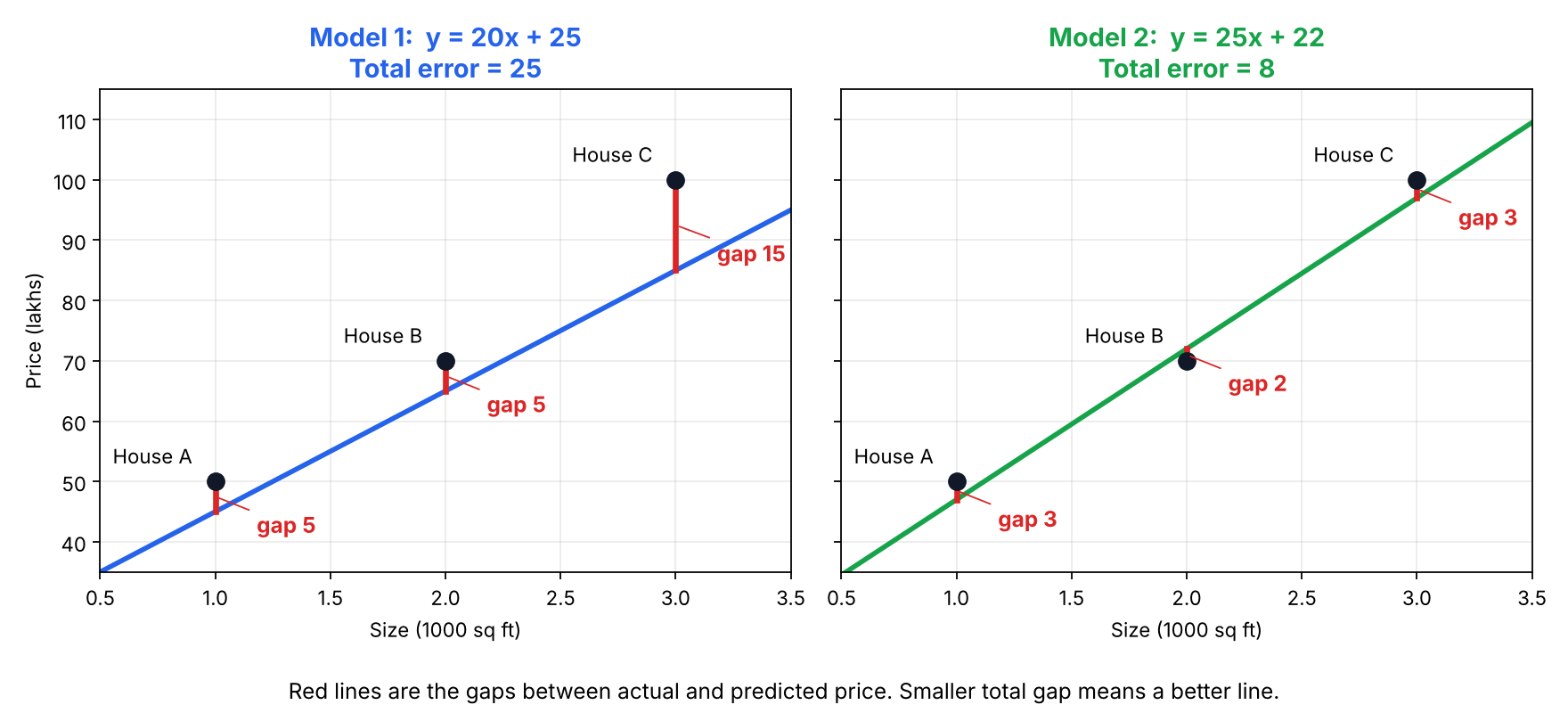
Since 8 < 25, Model 2 wins. Now we have a number to back it up, not just a feeling.

---

Wait, Why "Absolute"?

You may have noticed that we always treated the gap as positive. Here's why.

A line can predict too high (above the house) or too low (below it). If we kept the signs, the errors would cancel each other out:

+10 (too high)  +  (−10) (too low)  =  0

A terrible line could end up looking perfect! Taking the absolute value of each gap fixes this, so every miss counts, no matter which direction it's in.

---

So, What Is the Error Function?

That total sum of gaps is what we call the Error Function. You'll also hear it called the Loss Function or Cost Function. Same thing, different names.

Now think of it as a little game:

1. Start with a random line
2. Measure its error
3. Nudge the line (change m and c)
4. Measure again
5. Keep nudging in whichever direction reduces the error
6. Stop when the error can't get any smaller

The line you end up with is the best-fit line.

Big takeaway: "Training a model" simply means finding the m and c that make the error as small as possible.

🧮 The formula (don’t worry, it’s friendly)

Now let’s write what we’ve been doing in the language of mathematics. For the absolute error function, it looks like this:

$$E = \sum_{i=1}^{n} \left| y_i - \hat{y}_i \right|$$

Or, written in terms of our line ŷ = mx + c:

$$E(m, c) = \sum_{i=1}^{n} \left| y_i - (m x_i + c) \right|$$

It might look scary at first glance, but you don’t need to be scared of it. Look at it piece by piece and you’ll see it’s just a fancy way of writing the exact thing we already did by hand:

yᵢ is the actual price of the i-th house (what’s in our dataset). ŷᵢ (read as “y-hat”) is the predicted price from our line, which is just m·xᵢ + c. yᵢ − ŷᵢ is the gap between the actual and predicted price for that house. | | (the absolute value bars) make that gap positive, no matter which side of the line the house is on. Σ (sigma) simply means “add them all up”. i = 1 to n means “do this for every house, from the first one to the last one (n houses in total)”.

So in plain words, the whole formula says:

“For every house, find the gap between its actual price and the predicted price, make it positive, and add all those gaps together.”

That’s it! It is nothing but the sum of the differences we calculated in our tiny example. The formula is only shorthand, so we don’t have to write “gap of house A + gap of house B + gap of house C + ...” for thousands of houses.

The Error as a Valley

Here's a picture worth keeping in mind for the next article.

Change the slope m of our line (we keep c fixed here to keep the picture simple) and plot the total error each time. You get a valley:

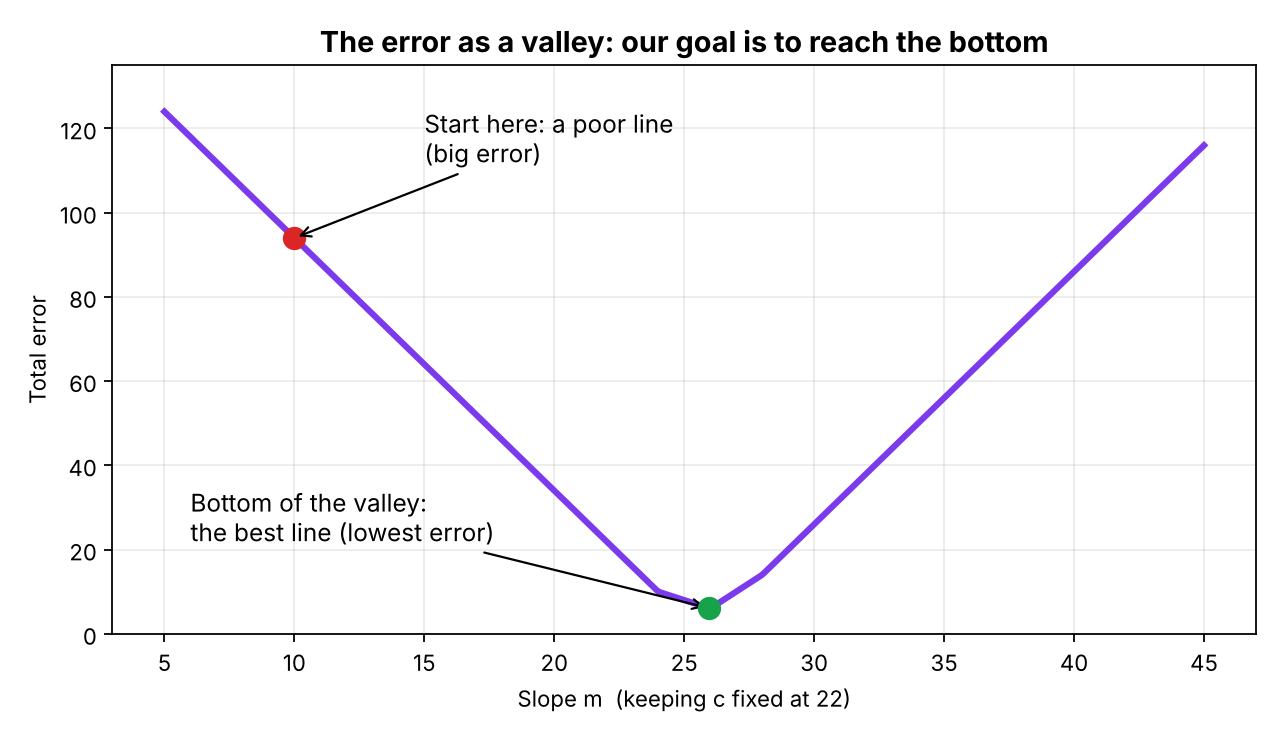
A poor line sits high up on the slope of the valley, with a big error. The best line sits at the very bottom. Our whole job is to walk down this valley until we can't go any lower.

Other Flavours of Error Functions

The one we used is called the Absolute Error. There are other popular ones too:

Error Function	What it does	Why people like it
Absolute Error (MAE)	Adds up the absolute gaps	Simple and easy to interpret
Squared Error (MSE)	Squares each gap	Punishes big misses harder and has a smooth curve, which is great for optimization
Root Mean Squared Error (RMSE)	Takes the square root of MSE	Brings the error back to the same units as the price

The job of every one of them is the same:

Measure how wrong the line is, so we can make it less wrong.

For this article, I used the absolute error because it's the easiest to understand. In the next article, we'll switch to squared error, because its smooth curve works beautifully with derivatives. Don't worry, the idea stays exactly the same.

🚀 What’s Next?

We now know how to score a line. But how do we actually find the best m and c without trying random lines forever?

Or to put differently: how do we walk down that valley and reach the lowest possible error?

To do that, we need to know which way is downhill at any point, and that is exactly what a derivative tells us. That's where Gradient Descent comes in, and we'll walk through it at the next stop in Algo City. 🏙️

Next Stop : Gradient Descent