The Moment Calculus Finally Made Sense: Gradient Descent Explained Simply

If you've read the previous articles and made it all the way here, thank you for the patience. Cheers! 🎉

In the last stop in Algo City, we learned how an error function tells us how good or bad our line is. That leaves us with the most interesting question of the series:

If our goal is to minimize the error, how do we actually find the $m$ and $c$ that give us the least error?

I mean, there are so many possible combinations of $m$ and $c$. How do we know which direction to move in? How does a machine figure out whether changing a value will improve its predictions or make them worse?

This is where Gradient Descent comes into the picture. And honestly, this is also where calculus finally started making sense to me.

---

🏔️ Welcome to Mount Descendra

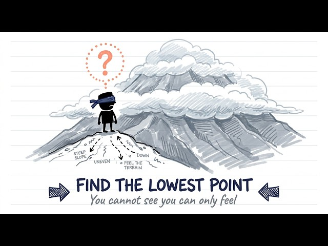
Imagine you're standing somewhere on a huge mountain called Mount Descendra. It's covered in thick fog, so you can't see the bottom. You have no idea where the lowest point is or how far away it might be. All you can observe is the ground right around you.

If your goal were to reach the bottom, what would you do?

You'd figure out which direction slopes downward, take a step, look around again, and repeat. One step at a time, until you reach a low point.

That's the basic intuition behind Gradient Descent.

But how does a mountain relate to our line in Algo City? Let's connect the dots.

---

📉 Remember the valley?

At the end of the last article, we plotted the error against the slope $m$ and got a valley. We kept $c$ fixed to keep the picture simple.

Now let's bring $c$ back. Every combination of $m$ and $c$ gives a different line, and so a different error. Put $m$ on one axis, $c$ on another, and the error on the vertical axis, and our valley grows into a whole landscape.

Every point on it is a line. Its height is the error. Higher means worse, lower means better.

Welcome to Mount Descendra. Our mission is to find the lowest point. 🎯

---

✏️ One small upgrade: squared error

Remember our promise from the last article? Time to switch from absolute error to squared error, because its curve is smooth (no sharp corners), and derivatives love smooth curves.

$$J(m, c) = \frac{1}{n} \sum_{i=1}^{n} \left( y_i - \hat{y}_i \right)^2, \qquad \hat{y}_i = m x_i + c$$

It's the same idea as before: find each gap, square it, add them all up, and divide by $n$ to take the average. Don't worry, nothing else changes.

---

🧭 How do we find our way down?

Back on the mountain, the fog hides the bottom, so we can't just look and pick the best path. But what if we could feel how steep the ground is under our feet?

If the ground rises as you step forward, you're going uphill. If it drops, you're going downhill. The slope tells you how the ground changes as you move.

This is exactly where calculus comes in.

A derivative tells us how a function changes when its input changes. Applied to our error function, it tells us how the error changes when we nudge $m$ or $c$:

$$\frac{\partial J}{\partial m} \qquad \text{and} \qquad \frac{\partial J}{\partial c}$$

Derivative	What it means
Positive	Increasing the parameter increases the error
Negative	Increasing the parameter decreases the error
Zero	The slope is flat at that point

For our squared error, these work out to:

$$\frac{\partial J}{\partial m} = -\frac{2}{n} \sum_{i=1}^{n} x_i \left( y_i - \hat{y}_i \right)$$

$$\frac{\partial J}{\partial c} = -\frac{2}{n} \sum_{i=1}^{n} \left( y_i - \hat{y}_i \right)$$

Together, these derivatives form the gradient:

$$\nabla J = \begin{bmatrix} \dfrac{\partial J}{\partial m} \[2mm] \dfrac{\partial J}{\partial c} \end{bmatrix}$$

Here's the important part: the gradient points in the direction of the steepest increase in error. Since we want to minimize the error, we walk in the opposite direction.

And just like that, calculus tells us which way to go on Mount Descendra. 🧗

---

👣 Taking the right step

Knowing which way is downhill is only half the story. We also need to decide how big a step to take.

Take huge steps and you might leap right past the lowest point. Take tiny steps and you'll get there eventually, but it could take forever.

The size of our step is controlled by the learning rate, written as \(\alpha\).

Learning rate	What happens
Too small 🐢	Safe, but painfully slow
Just right ✅	Steady progress toward the minimum
Too large 🚀	Overshoots, bounces around, or even diverges

Now let's translate our mountain journey into mathematics:

$$m_{\text{new}} = m_{\text{old}} - \alpha \frac{\partial J}{\partial m}$$

$$c_{\text{new}} = c_{\text{old}} - \alpha \frac{\partial J}{\partial c}$$

Notice that minus sign? That's the key. It tells us to move opposite to the gradient.

After each update, we measure the error again, look at the new gradient, and take another step. We repeat this until the error is as small as we can make it.

---

🏙️ Let's take one step in Algo City

Same three houses from the last article (size in 1000 sq. ft., price in ₹ lakhs):

House	Size (x)	Actual Price (y)
A	1	50
B	2	70
C	3	100

We start with our old Model 1: \(m = 20\), \(c = 25\), and choose a learning rate \(\alpha = 0.05\).

House	Predicted	Actual	Gap (\(y - \hat{y}\))
A	45	50	5
B	65	70	5
C	85	100	15

Error: \(J = \dfrac{5^2 + 5^2 + 15^2}{3} \approx 91.7\)

Now the slopes of our landscape at this point:

$$\frac{\partial J}{\partial m} = -\frac{2}{3}\left(1 \cdot 5 + 2 \cdot 5 + 3 \cdot 15\right) = -40$$

$$\frac{\partial J}{\partial c} = -\frac{2}{3}\left(5 + 5 + 15\right) \approx -16.7$$

🧠 Both slopes are negative, which means increasing $m$ and $c$ will reduce the error. So let's step:

$$m_{\text{new}} = 20 - 0.05 \times (-40) = 22$$

$$c_{\text{new}} = 25 - 0.05 \times (-16.7) \approx 25.8$$

Our new line is \(y = 22x + 25.8\), and its error drops from 91.7 to about 23.8. One step, and we're already much lower on the mountain! 🎉

Keep repeating, and the line settles near \(m = 25\) and \(c \approx 23.3\), which is right around the Model 2 we found by hand last time.

⚠️ Gradient Descent doesn't guarantee that every problem leads to the global minimum. It depends on the shape of the error function, the learning rate, and other factors. (For Linear Regression with squared error, the landscape is a single smooth bowl, so we're in good shape!)

The central idea stays simple: use the gradient to understand how the error changes, then update the parameters in the opposite direction.

---

✨ And that's Gradient Descent!

When I first met calculus, derivatives felt like formulas I had to memorize and apply. I could work through the equations, but I didn't always understand what they were actually telling me.

Thinking of derivatives as slopes changed that. Thinking of gradients as directions made it even clearer. And imagining Gradient Descent as a journey down Mount Descendra connected the mathematics to something I could actually picture.

Suddenly, those equations weren't just symbols on a page. They described a process I could understand.

And maybe that's one of the most beautiful things about mathematics: sometimes all we need is the right way to look at a concept for everything to click.

---

🎬 Our journey through Algo City

Stop	What we learned
The Big Picture	Linear Regression finds the best-fitting line
The Error Function	We can measure how good or bad a line is
Gradient Descent	We can use slopes to make the line better, step by step

We don't need to see the entire mountain to begin our journey. We just need to understand the slope around us, take a step in the right direction, and keep going.

One step at a time, until we find our way down Mount Descendra. 🏔️

---

📝 One last note before you go

In this series we used just two parameters, $m$ and $c$, so we could actually picture the mountain. But when you move on to real ML models and see the formulas in the wild, you'll find many more parameters, often written as \(\theta_1, \theta_2, \dots, \theta_n\). Some models have thousands or even millions of them.

Don't let that confuse you. The update rule just repeats for every parameter:

$$> \theta_j = \theta_j - \alpha \frac{\partial J}{\partial \theta_j} >$$

The landscape gets bigger, but the intuition stays exactly the same: feel the slope, step the opposite way, repeat. 🏔️

---

💬 If this explanation helped Gradient Descent click for you, I'd love to hear your thoughts. And if there's another mathematical concept that finally made sense to you through a real-world analogy, share it in the comments!