Linear Regression: Understanding the Big Picture

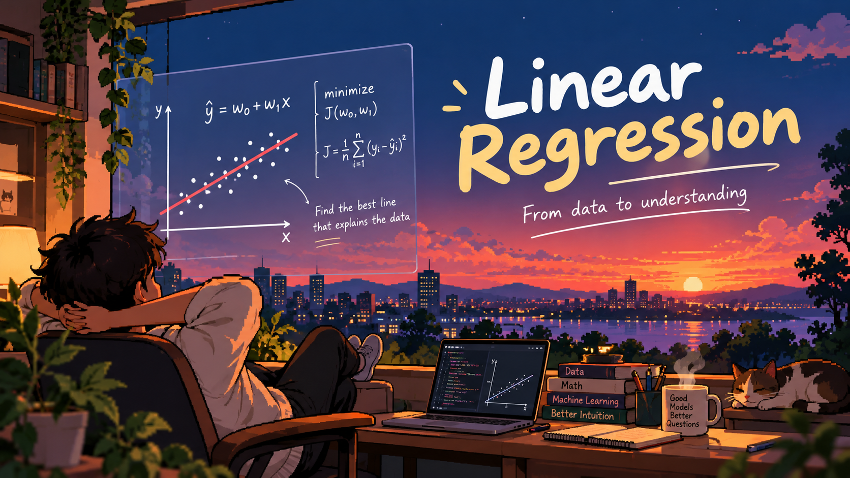
What is Linear Regression?

Before diving into the mathematics, let's first understand what Linear Regression actually means in simple terms — something that anyone can understand, regardless of their mathematical background.

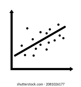
Imagine you have a bunch of data points scattered across a graph. Our goal is to find a straight line that fits these points as closely as possible.

That's the basic idea behind Linear Regression.

In simple terms, Linear Regression tries to find the best-fitting straight line for a given dataset, so that the predictions made by the line are as close as possible to the actual data points.

Take a look at the image below. It should give you a visual intuition of what we're trying to achieve before we dive into the mathematics behind it.

A House in Algo City 🏡

Imagine a city called Algo City, where every house has its own story and, of course, its own price!

Now, suppose you're planning to buy a house in this city. Naturally, one of the first things you'd want to know is:

💭 How much would a particular house cost?

You start exploring the city and collecting information about houses that have already been sold. As you look at the data, you notice something interesting: the size of a house seems to have a relationship with its price. In general, larger houses tend to cost more, while smaller houses tend to cost less.

Let's look at some data you've collected from Algo City. 📊

House	Size (sq. ft.)	Price (₹ lakhs)
House A	500	25
House B	800	40
House C	1,000	50
House D	1,200	60
House E	1,500	75

🧠 Let's put on our thinking caps!

Take a moment to look at the data above.

If I ask you to predict the price of a 1,100 sq. ft. house, how would you do it?

Interestingly, some of you might have already spotted a pattern! 👀

For every additional 100 sq. ft., the price increases by ₹5 lakhs. The price increases proportionally with the area of the house.

So, we can use this pattern to estimate the price of a house we've never seen before.

Some of you, especially those with a mathematical background, might have already gone a step further and expressed this relationship using a mathematical equation:

[y = 0.05x]

Here:

• (x) represents the area of the house in square feet.
• (y) represents the predicted price in lakhs of rupees.

Let's put our equation to the test! 🚀

For a house with an area of 1,100 sq. ft.:

[y = 0.05 \times 1100 = 55]

🎯 Our predicted price is ₹55 lakhs!

Pretty cool, right? We started with a collection of houses and their prices, spotted a pattern, and expressed that pattern mathematically.

And that's the fundamental idea behind Linear Regression: finding a mathematical relationship between our inputs and outputs so that we can make predictions.

---

🤔 But what happens when things aren't so simple?

Our example was quite straightforward. The data followed a perfect pattern, making it easy to identify the relationship just by looking at the numbers.

But real-world data is rarely this perfect!

Imagine collecting information about hundreds of houses in Algo City. Some houses might be more expensive because they're in better neighbourhoods. Others might have different amenities, be newer, or be closer to schools and offices.

As a result, two houses with exactly the same area might have completely different prices.

If we plot all these houses on a graph, we probably won't see every point falling neatly along a straight line.

So, here's the challenge. 💡

How do we find a straight line that captures the overall relationship between the area and the price of these houses?

We could draw a line ourselves, but how would we know if it's a good one? What if another line makes predictions that are closer to the actual prices?

And if we want a computer to do this for us, how can we teach it to find a suitable line on its own?

⚙️ The basic idea behind Linear Regression

Let's break it down into three simple steps:

1️⃣ Start with a line

We begin with an initial guess for a straight line, represented by the equation:

[y = mx + c]

2️⃣ Adjust the line

We change the values of (m) and (c) to make the line fit our data points more closely.

3️⃣ Repeat and improve

We repeat this process over multiple iterations, gradually improving the line until we find one that fits the data as well as possible.

In simple terms, we start with a line and try to make it better and better at predicting the prices of houses. 📈

🤔 But how do we know if our line is actually good?

And more importantly, how do we decide how to adjust (m) and (c) to improve it?

That's where things get interesting!

In the next article, we'll explore the Error Function and understand how we can mathematically measure how good or bad our line is.

👉 Continue reading: Linear Regression: Understanding the Error Function